Incidence rate-difference models

fludta <- flumodelr::fludta

Introduction to incidence rate-difference models

Incidence rate-difference models are among the first to estimate influenza-associated hospitalizations and deaths (Izurieta HS 2000). In these models incidence rates in periods with low viral activity are substracted from incidence rates in periods with high viral activity. This difference in incidence rate is assumed to be influenza attributable.

Virology data

To determine periods with high and low viral activity, researchers often use laboratory confirmed influenza data or the percent of isolates positive with influenza viral types. This is publically available in many cases, see ?nrevss for US surveillance data. The data describes the proportion of isolates tested positive for a certain viral type, which may be obtained from participating hospital and outpatient settings.

Definition of periods: default values

We followed Thompson (Thompson WW 2009) and defined the respiratory season to start at the beginning of July (week 27) of each calendar year. Within a respiratory season we defined four periods:

a high viral activity period consisting of weeks when at least 10% of specimens are positive,
a peri-season baseline period consisting of weeks when less than 10% of specimens were positive, and;
an influenza season defined as the weeks from October (week 40) through April (week 18),
a summer-season baseline period defined as the weeks from July (week 27) through September (week 39) at the beginning of each respiratory season and May (week 19) and June (week 26) at the end of each respiratory season when there is little viral activity.

Options c and d can be used in the absense of laboratory confirmed influenza surveillance data to define high and low viral activity periods.

Annual excess numbers

Weekly excess outcome rates will be converted to annual excess numbers of outcomes by using the number of weeks that were above an epidemic threshold, and available US census data:

annual excess [outcomes] = (excess weekly rate) x (number of epidemic weeks) x (population).

Example: peri-season adjusted influenza attributable mortality

In this example we will estimate influenza attributable mortality using a peri-season adjustment. We will adjust mortality in weeks with high viral activity (a) with weeks when viral activity was low (b). All we have is a dataset with surveillance data (‘prop_flupos’) in a certain calendar ‘year’ and ‘week’, plus the observed number of all cause hospitalizations in that week (‘alldeaths’).

We remove years without viral activity

df <- fludta %>% 
  dplyr::filter(year>2010 & year <2016) %>%
  select(year, week, alldeaths, prop_flupos, week)

Step 2. ird() function

fludta_mod <- ird(data =df, 
                  outc =alldeaths, 
                  viral=prop_flupos, 
                  time =week,
                  echo =T)
#> incidence rate-difference model 
#>  ============================================================ 
#> Setting ird parameters...
#>  'outc' argument is: alldeaths 
#>  'time' variable is: week 
#>  'viral' variable is: prop_flupos 
#>  'high' variable is: 0.1 
#>   time period is: 52

The initial function prepares the dataset by identifying periods of high and low viral activity in the respiratory season. It creates the table fludta_mod, adding 3 varables (columns): respiratory ‘season’, ‘high[,“prop_flupos”]’ (TRUE = high viral activity, FALSE = low viral activity), and ‘fluseason’ (TRUE = flu season, FALSE = summer-season baseline)

fludta_mod %>% select(year, week, alldeaths, 
                      prop_flupos, week, season, high, fluseason)
#> # A tibble: 261 x 7
#>    year  week alldeaths prop_flupos season high[,"prop_flupos"] fluseason
#>   <int> <int>     <int>       <dbl>  <dbl> <lgl>                <lgl>    
#> 1  2011     1     13291      0.239    2010 TRUE                 TRUE     
#> 2  2012     1     10906      0.0334   2011 FALSE                TRUE     
#> 3  2013     1     11258      0.374    2012 TRUE                 TRUE     
#> 4  2014     1     11070      0.281    2013 TRUE                 TRUE     
#> # ... with 257 more rows

Note that ‘high[,“prop_flupos”]’ will not be created if ird(viral= missing).

Step 2. rb() function

fludta_rates <- rb(data =fludta_mod, outc =alldeaths, echo = T)
#> Setting rb parameters...
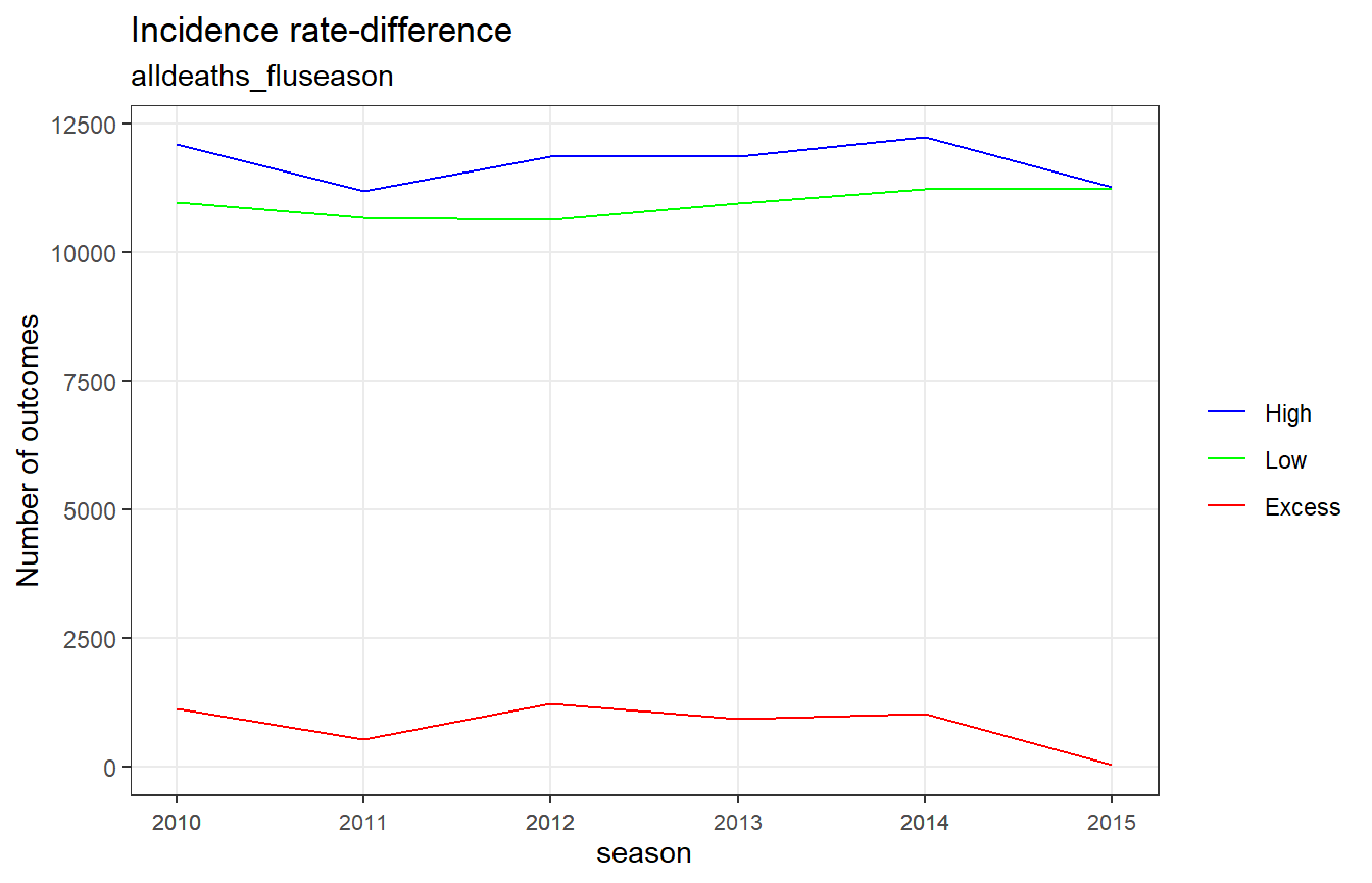
#>  'outc' argument is: alldeaths

The rb() function aggregates the outcomes per time period (weeks in our example) to outcomes per respiratory season, stratified by period of high and low viral activity, and excess rates (period = “High” - period = “Low”).

fludta_rates
#> # A tibble: 18 x 4
#>   season period alldeaths_fluseason alldeaths_viral_act
#>    <dbl> <fct>                <dbl>               <dbl>
#> 1   2010 Excess               1133.               1172.
#> 2   2010 Low                 10982.              11046.
#> 3   2010 High                12116.              12218.
#> 4   2011 Excess                519.                155.
#> # ... with 14 more rows

For ‘alldeaths_fluseason’, ‘period’ is defined by flu season (High = flu season, Low = summer-season baseline) For ‘alldeaths_viral_act’, ‘period’ is defined by viral activity (High = high viral activity, Low = low viral activity)

Note that ‘alldeaths_viral_act’ will not be created if ird(viral= missing).

Generate figure

gr(data =fludta_rates, outc =alldeaths_fluseason, echo = FALSE )

References

Izurieta HS, Kramarz P, Thompson WW. 2000. “Influenza and the Rates of Hospitalization for Respiratory Disease Among Infants and Young Children.” N Engl J Med 342: 232–39.

Thompson WW, Dhankar PY, Weintraub E. 2009. “Estimates of Us Influenza-Associated Deaths Made Using Four Different Methods.” Influenza Other Respir Viruses 3(1): 37–49.

Rob van Aalst

2019-06-06